DirectProbe-Studying Representations without Classifiers

Analyze the geometry of representions.

Direct Probe v.s. Classifier Proxy Probe

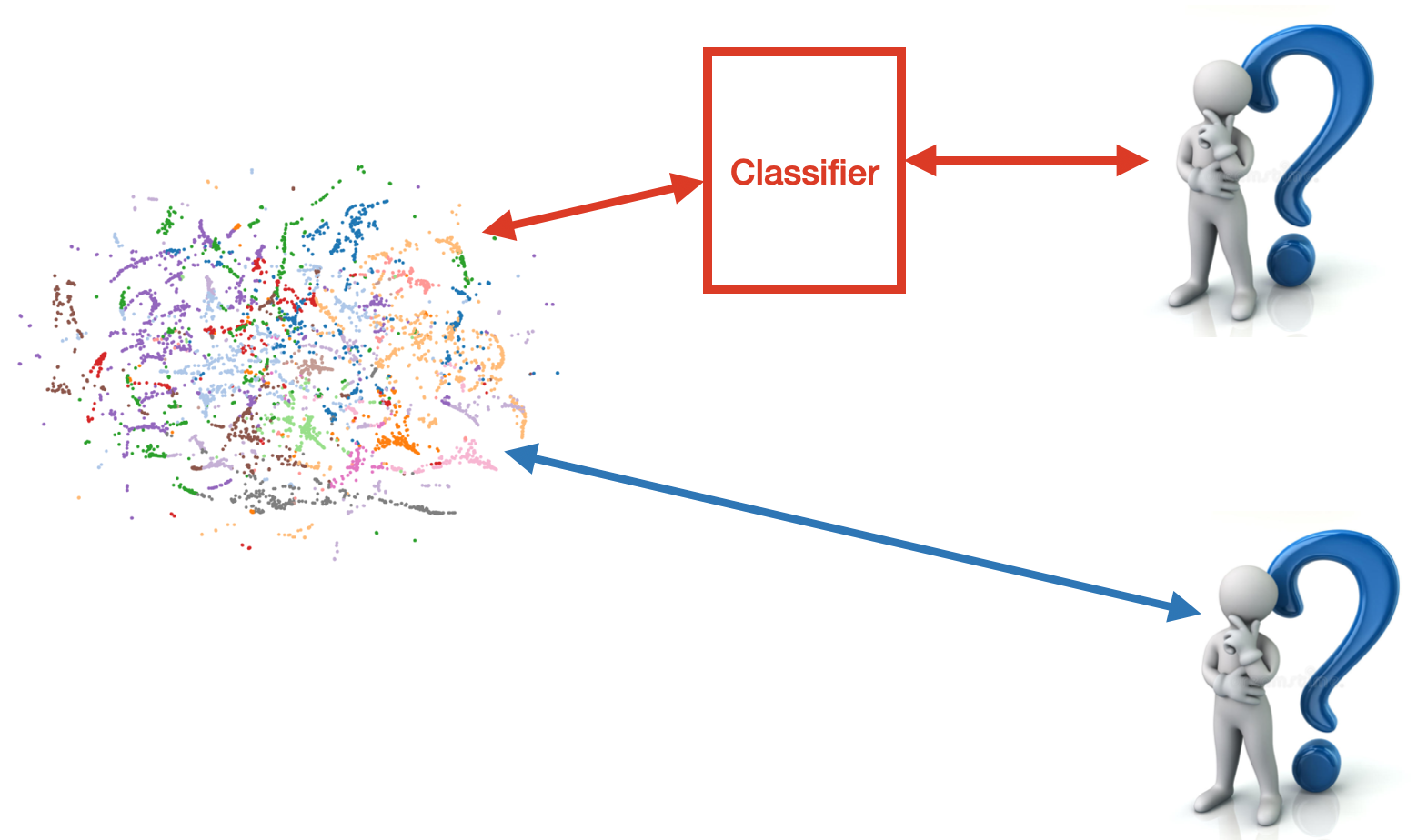
Understanding the representation space is a hot topic in the area of NLP since distributed representations made huge improvments on variety of NLP tasks and we do not know why. Exisiting probing methods use a learned classifier’s accuracy, mutual information or complexity as a proxy for the quality of a representation. However, classifier-based probes fail to reflect the difference because different representations may require different classifiers. In this post:

• We argue that training classifiers as probes are not reliable. Instead, we should directly analyze the structure of representations;
• We introduce the notion of \(\epsilon\)-version space which can serve as a distinugished characteristic of a representation;
• We propose DirectProbe, a heuristic probing method to approximate \(\epsilon\)-version space and anlayze representation space without training classifiers;
• We show that results of DirectProbe can explain the different classifier behaviors of representations.

Why Classifier-based Probing not Reliable

A learning task can usually be decomposed into three components:

1. The problem itself, which consists of the task and the dataset. For example, Part-of-Speech tagging is a task and Penn Treebank is a dataset.
2. A learning process, which consists of the model, algorithm and loss functions. For example, we can predict the POS tags by training a two-layers neural netowork (model) with cross-entropy loss (loss function), which can be optimized by AdamW (algorithm).
3. Representation, which projects the input objects into a feature space. This feature space is usually a high dimensional vector space. For example, a token in one sentence can be mapped to a 768 dimension vector by BERT model.

Learning components and their factors

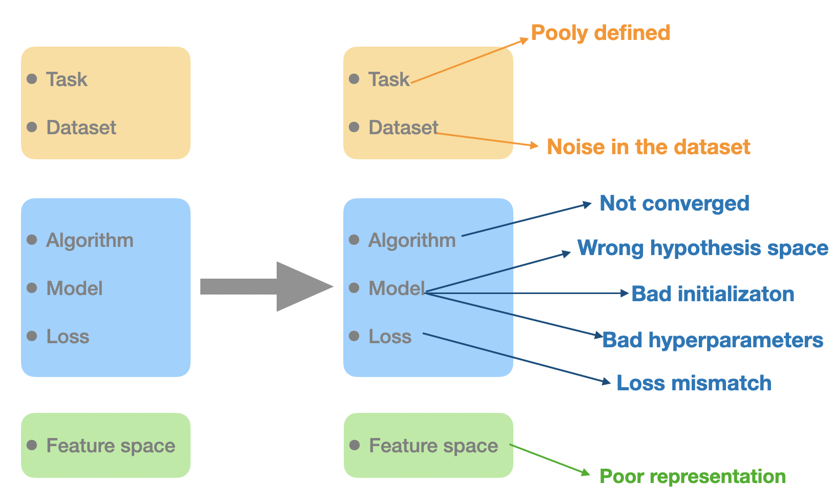
However, there are so many factors can affect the performance of the whole learning process. For example, the optimizer (the algorithm) stops before convergence or we choose a bad initialization point. The above figure list all the possible factors. Clearly, the quality of the representation space is not the only factor.

Preliminary experiments are conducted on the supersense role labeling task with BERT-base-cased and ELMo original model. Many different classifiers are trained and evaluated, from logistic regression to two layer neural network. For each specific classifier, we train for \(10\) times using \(10\) different random seeds and record the minimum and maximum accuracy for these \(10\) runs. The following table shows our initial experiment results.

Inital experiments on supersense role labeling task

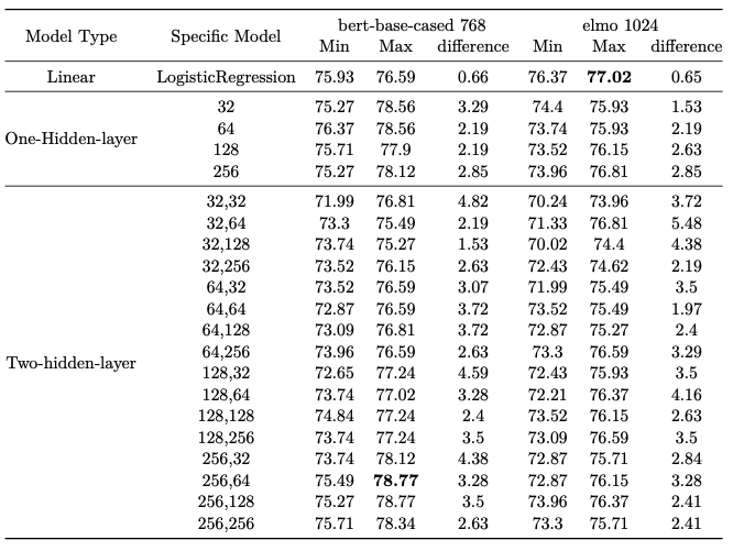
From the table above, we observe:

• Even only the random seed is different (each row in the table), the accuracy difference between learned classifiers can be as large as \(3\) or \(4\) percent, which is non-ignorable.
• Different representations require different model architectures to acheive the best performance. For example, BERT-base-cased requires a two-layer neural network whose hidden sizes are \(256\) and \(64\), while ELMo requires a simple linear model.

The above figure and table show that evaluating the quality of representations based on the learned classifiers is not reliable. Bad initialization point or wrong choice of model type can also lead to a bad predictive performance. We can conclude that a bad predictive performance does not necessarily mean bad representation and vice versa.

In this post, we study the question: Can we evaluate the quality of a representation for an NLP task directly witout relying on classifiers as proxy?

\(\epsilon\)-Version Space: The Characteristic of a Representation

Given an NLP task, we want to distentangle the evaluation of a representation \(E\) from the classifier \(h\) that are trained over it. To do so, the first step is to characterize all classifiers supported by a representation.

From the viewpoint of a classifier, it is trained to find a set of parameters such that the prediction of the classifier is consistent with the examples in the training set. Geometrically speaking, each learned classifier is a decision boundary in the high dimension space as showed in the following figure.

Decision boundaries admitted by a representation

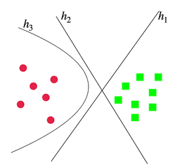
In the above figure, it is a simple binary classification problem. There are many classifiers that can separate these two classes. This figure shows two linear (\(h_1\) and \(h_2\)) and a non-linear (\(h_3\)) examples. This suggests us that a representation $E$ can admit a set of classifiers that are consistent with the training set and a learner choose one of them. Given a set \(\mathcal{H}\) of classifiers of interest, the subset of classifiers that are consistent with a given dataset represents the version space with respect to \(\mathcal{H}\). However, the original definition of version space does not allow errors. Here, to account for the errors or noise in the data, we define a \(\epsilon\)-version space: the set of classifiers that can achieve less than \(\epsilon\) error on a given dataset.

Suppose \(\mathcal{H}\) is the whole hypothesis space consisting of all possible classifiers \(h\) of interest. The \(\epsilon\)-version space \(V_{\epsilon}(\mathcal{H}, E, D)\) expressed by a representation \(E\) for a labeled dataset \(D\) is defined as:

\[V_{\epsilon}(\mathcal{H}, E, D)\triangleq \{h\in \mathcal{H}\vert err(h, E, D)\le \epsilon\}\]

where \(err\) is training error.

Be note here, the \(\epsilon\)-version space \(V_{\epsilon}(\mathcal{H},E,D)\) is only a set of learned classifiers and does not involve any learning. Intuitively, the larger \(\epsilon\)-version space would make the learning process easier to find a consistent classifier.

Connection to Previous Work

Previous classifier-based probing work measures the quality of a representation by investigating properties of a specific \(h\in V_{\epsilon}\). For example, some work restricts the probe model to be linear. Commonly measured properties include generalization error , minimum description length of labels and complexity . Different from previous work, we seek to directly evaluate the \(\epsilon\)-version space of a representations for a task, without committing to a restricted set of probe classifiers.

DirectProbe: Approximating \(\epsilon\)-Version Space by Clustering

Now, the next question is how can we find the \(\epsilon\)-version space for each representation. From the definition, \(V_{\epsilon}(\mathcal{H},E,D)\) is a infinite set. Although it is impossible to enumerate all the possible classifiers, geometry perspective indeed provide some insights about \(V_{\epsilon}(\mathcal{H},E,D)\).

Mimic Decision Boundaries

We know that each classifier \(h\in V_{\epsilon}(\mathcal{H},E,D)\) is a decision boundary in the representation space and it can be in the form of any shape, like the following figure shows. On the left, the decision boundaries can be linear or non-linear. On the right, the decision boundary has to be a circle.

Using piecewise functions to mimic decision boundaries

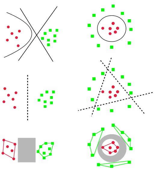
We also know that a set of piecewise linear functions can mimic any functions. If we use a set of piecewise linear functions to mimic the decision boundaries (the middle ones in the above figure), we find that the space is split into different groups, each of which contains points with exactly one label. Because of linear functions, these groups are seen as convex regions in the representation space (the bottom ones in the above figure). Any classifier in \(V_{\epsilon}(\mathcal{H},E,D)\) must cross the region between the groups with different labels; these are the regions that separate labels from each other, as shown in the gray areas in the bottom of above figure. So, an intuitive idea is to use these grey areas to approximate the \(V_{\epsilon}(\mathcal{H},E,D)\).

Clustering

Although finding the set of all decision boundaries remain hard, finding the regions between convex groups that these piecewise linear function splits the data into is less so. Grouping points in the space is well-defined problem: Clustering. However, in this case, our clustering problem has different criteria:

• All points in a group must have the same label. We need to ensure we are mimicking the decision bounaries.
• There are no overlaps between convex hulls of each group. If convex hulls of two groups do not overlap, there must exist a line that can separate them, as guaranteed by the hyperplane separation theorem.
• Minimize the number of total groups. Otherwise, a simple solution is that each data point becomes a group by itself.

Now, we successfully transform the problem of finding \(\epsilon\)-version space into a clustering problem with special criteria.

DirectProbe: Heuristic Clustering

To find clusters that satisify the above criteria, we propose DirectProbe, a simple yet effective heuristic clustering algorithm:

• Initiaize each point to be a cluster
• Always pick two closest clusters to be merged
• Two clusters can be merged only when
  • They have the same label
  • The convex hull of new cluster does not overlap with convex hulls of other clusters
• Repeat until no clusters can be merged

Animation of DirectProbe

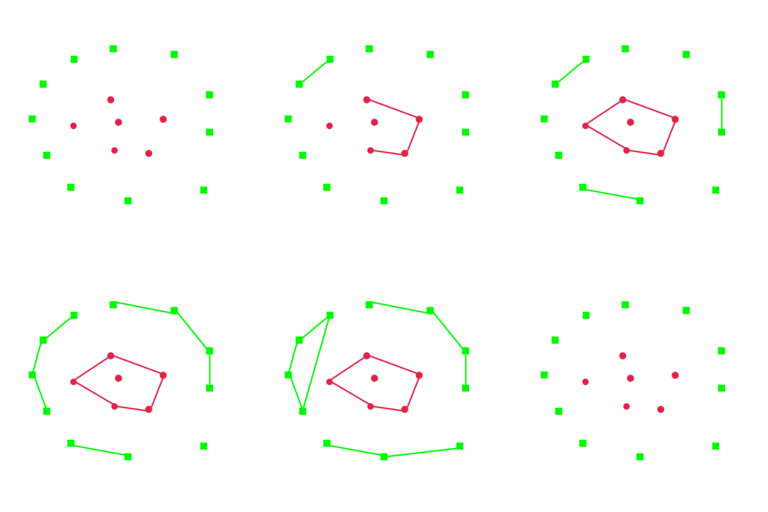
The above animation describes the algorithm. When the new cluster overlaps (green dashed lines) with the red ones, it stops the merging and find the next closest pair.

Applications of the Clusters

Now, we have developed DirectProbe, a heuristic clustering approach that can approximate \(\epsilon\)-version space. Next, we apply this approach on variety of representations and tasks and analyze the results.

Number of Cluster Indicate Linearity

After applying the DirectProbe, we could end up \(n\) clusters.

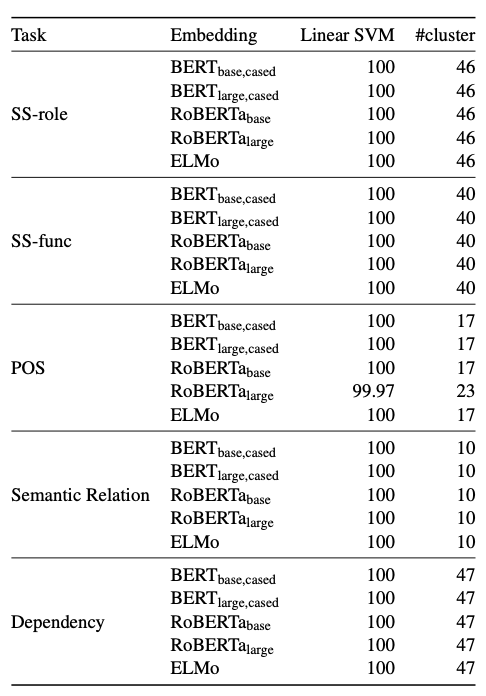
• If \(n\) equals to the number of labels, examples with the same label are placed close enough by the representation to form a cluster that is separable from other clusters. In this scenario, a simple linear multi-class classifier can fit well.
• If \(n\) is larger than the number of label, then some labels are distributed across multiple clusters. This means the decision boundary that can separate the clusters is non-linear. Consquently, this scenario calls for a more complex classifier, e.g. a multi-layer neural network.

By using the number of clusters, we can answer the question:

Can a linear classifier fit the training set for a task with a given representation?

To validate our claim, we use the training accuracy of a linear SVM classifier. If a linear SVM can perfectly fit (\(100\%\) accuracy), then there exist linear decision boundaries that separate the labels. The following table shows the results of our experiments. We can observe that almost all of the representations we experimented are linear separable for most of the tasks. We think this maybe the reason why linear model usually work for BERT-family models. The only exception is RoBERT-large on the pos tagging task. DirectProbe ends up with \(1487\) clusters and linear SVM can not achieve \(100\%\) training accuracy either.

Be note, linear separability does not mean the task is easy or that the best classifier should be a linear one.

Linearity of different representations and tasks

Higher Layers have larger \(\epsilon\)-Version Space

The distance between clusters is another important property we should consider. We apply the DirectProbe on each layer of BERT-base-cased model for five tasks. For each layer(space), we compute the minimum distance between all pairs of clusters. The next figure shows our results.

Minimum distances between clusters v.s. the best classifier accuracy

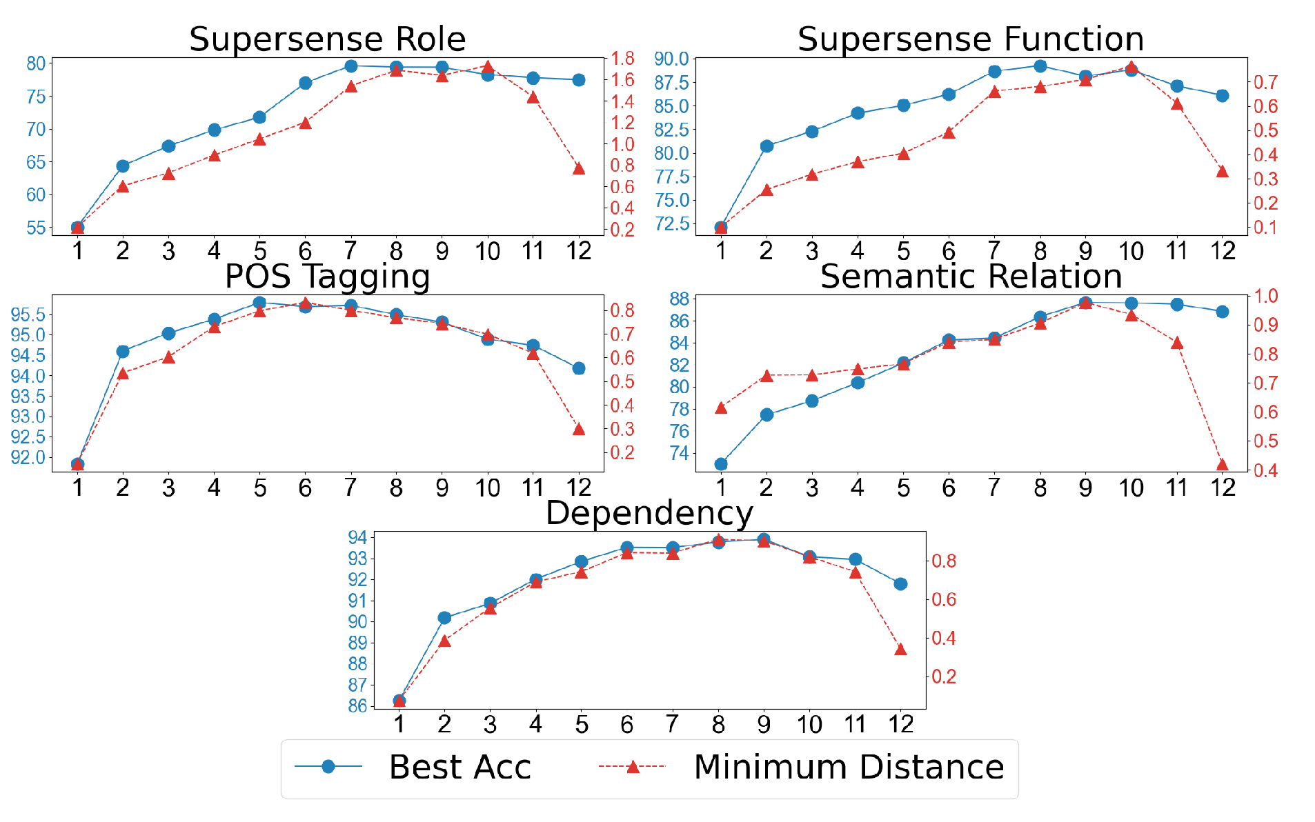
The horizonal axis is the layer index of BERT-base-cased, the left vertical axis (blue line) is the best classifier accuracy and right vertical axis (red line) is the minimum distance between all pairs of clusters. We observe that both best classifier accuracy and minimum distance show similar trends across different layers: first increasing, then decreasing. Although not a simple linear relation, it shows that minimum distance correlates with the best performance for an embedding space. Using the minimum distances of different layers, we answer the question:

How do different layers of BERT differ in their representations for a task?

Fine-tuning expands the \(\epsilon\)-Version Space

The standard pipeline of using contextual embedding models is to fine-tuning the original model on a specific task and then deploy fine-tuned model. Fine-tuning usually can improve the performance, which makes us wondering:

What changes in the embedding space after fine-tuning?

We apply the DirectProbe on the last layer of BERT-base-cased before and after fine-tuning for five tasks. Similarily, we compute the minimum distances between all pairs of clusters. The next table shows the results.

The best performance and the minimum distances betweeen all pairs of clusters of the last layer of BERT-base-cased before and after fine-tuning.

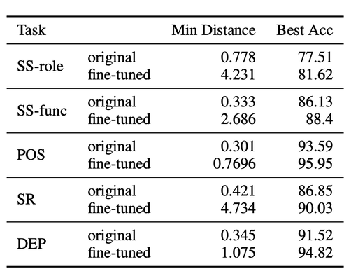
We can observe that both the best classifier accuracy and minimum distance show a big boost. It means that fine-tuning pushes the clusters away from each other in the representation space, which results in a larger \(\epsilon\)-version space. This verifies our assumption:

A larger $\epsilon$-version space admits more classifiers and allows for better generalization

Small Distances Confuses Classifiers

The distance between clusters can also confuses classifiers. By comparing the distances between clusters, we answer the question:

Which labels for a task are more confusable?

We compute the distances between all pairs of labels based on the last layer of BERT-base-cased¹. The distances are evenly split into 3 categories: small, medium and large. We partion all label pairs into these three bins. For each task, we use the predictions of the best classifier to compute the number of misclassified label pairs for each bin. The distribution of all errors is shown in the following table.

Error distribution based on different distance bins. The number of label pairs in each bin is shown in the parentheses.

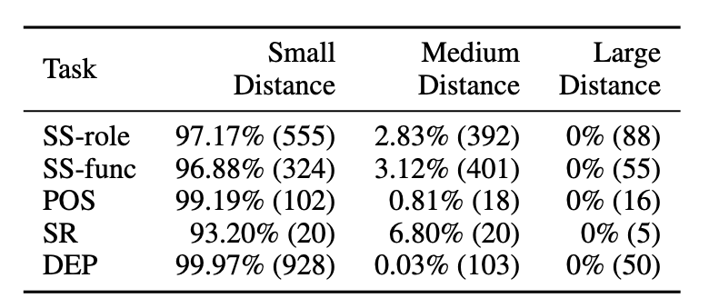
We can easily observe that all the errors concentrate on the small distance bin. This means that small distance between clusters indeed confuse a classifier and we can detect it without training classifiers.

Predict Expected Performance of the Best Classifier

As we discussed earlier, any classifier \(h\in V_{\epsilon}(\mathcal{H},E,D)\) is a predictor for the task \(D\) on the representation \(E\). So, as a by-product, the clusters from DirectProbe can also be used as a predictor. The prediction strategy can be very simple: for a test example, we assign it to its closest cluster. We call this accuracy intra-accuracy. Because this strategy is very similar to the nearest neighbor classification (1-kNN), which assigns the unlabeled test point to its closest labeled point, we also compare with the 1-kNN accuracy. The following figure shows the results.

Comparison between the best classifier accuracy, intra-accuracy and 1-kNN accuracy. The X-axis is different representation models. BB:BERT-base-cased, BL:BERT-large-cased, RB: RoBERT-base, RL: RoBERT-large, E: ELMo. The pearson correlation coefficient between best classifier accuracy and intra-accuracy is shown in the parentheses alongside each task title.

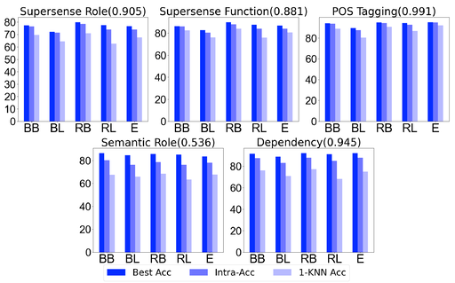
We observe that intra-accuracy always outperforms the simple 1-kNN classifier, showing that DirectProbe can utilize more information from the representation space. Moreover, all the pearson correlation coefficients between best accuracy and intra-accuracy (showed in the parentheses alongside each task title) suggests a high linear correlation between best classifier accuracy and intra-accuracy, which means the intra-accuracy can be a good predictor of the best classifier accuracy for a representation. From this, we argue that intra-accuracy can be interpreted as a benchmark accuracy of a given representation without actually training classifiers.

Conclusion

In this post, we ask the question: what makes a representation good for a task? We answer it by developing DirectProbe, a heuristic approach builds upon hierarichal clustering to approximate the \(\epsilon\)-version space. By applying DirectProbe, we find:

• The number of clusters can indicate the linearity of the representation space.
• For BERT model, the higher layers have larger \(\epsilon\)-version space.
• Fine-tuning can expand the \(\epsilon\)-version space, which leads to a better generalization.
• DirectProbe can also predict the expected best classifier performance.

linearly separable. So the number of labels pairs equals the numebr of cluster pairs.

1. For all tasks, the last layer of BERT-base-cased is ↩