How Fine-tuning Changes BERT

Analyze how fine-tuning changes BERT representation.

Fine-tuning

The standard pre-training—fine-tuning setting, borrowed from Ruder's blog

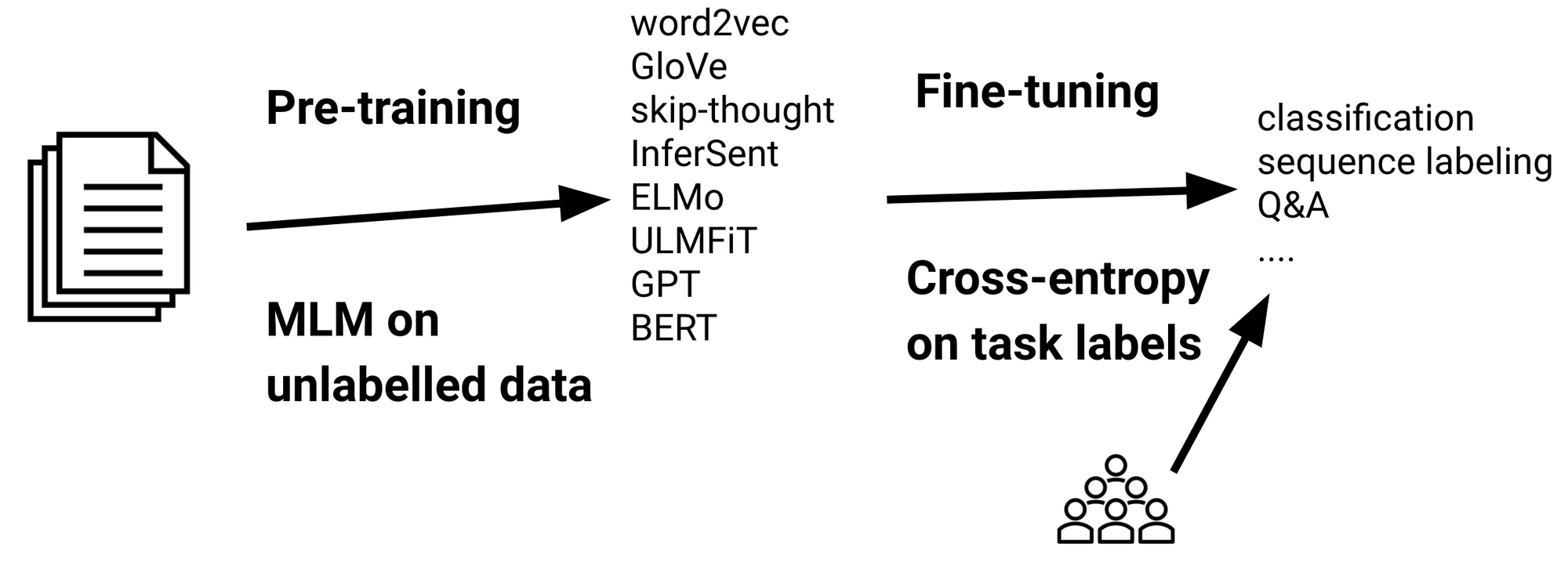
Fine-tuning a pre-trained model on a specific task becomes a standard strategy to improve the task performance. However, very little is understood about how fine-tuning process affects the underlying representation and why fine-tuning invariably seems to improve the performance.

We applied two probing methods, classifier-based probing and DirectProbe on variants of BERT representations and tasks. In this post,

• We show that fine-tuning introduces a divergence between training and test sets. We also discover one exception where fine-tuning hurts the performance.
• We reveal two reasons why fine-tuning can improve the performance: (i) Fine-tuning adjusts the representation such that it groups points with the label into a smaller number of clusters (ideally one); (ii) Fine-tuning pushes the clusters of points representing different labels away from each other, producing a larger separating regions between labels.
• By investigating the effect of across tasks fine-tuning, we verify the hypothesis that fine-tuning improve the task performance by altering the distances between label clusters.
• We show that lower layers do change during the fine-tuning, but to a much lesser extent than the higher ones.

Probing methods

To analyze how fine-tuning works, we use two probing methods to analyze the represention space before and after fine-tuning process.

Classifiers as Probes

The first probe we used is a classifier-based probe, which is a common methodology to probe representation space. We train classifiers over representations to understand how well a representation encodes the labels for a task. For all of our analysis, we use two-layer neural networks as our probes. The classification performance can provide a direct assessment of the effect of fine-tuning.

DirectProbe: Probing the Geometric Structure

The second probe we used is DirectProbe, a recently proposed technique which analyzes representation space from a geometric perspective by clustering. Different from the other probes that analyze the geomtry of the representations, DirectProbe requires a representation and a given labeling task. It is reasonable to probe the representation based on a give task because fine-tuning a representation creates different representations for different tasks.

DirectProbe is built on upon the categorizetion of not one, but all decision boundaries in a representation space that are consistent with the a training set for a given task. It approximates this set of decision boundaries by a supervised clustering algorithm, which returns a set of clusters such that each cluster only contains the points with the same label. There are no overlaps between the convex hulls of these clusters. The following figure describe this process. More detailed description of DirectProbe can be found here.

Clustering illustration of DirectProbe: red circle and green square are two classes

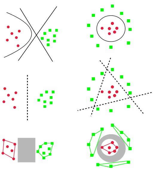
We use three properties of the clusters returned by DirectProbe to measure the representations:

1. Number of Clusters. The number of clusters can indicate the linearity of the representation for a task. If the number of clusters equal to the number of labels, then all the examples with the same label are grouped into the one cluster (left example in the above figure). One linear classifier is sufficient to describe the decision boundaries. In contrast, if the number of clusters are greater than the number of labels, then there are at least two clusters with the same label can not be grouped together (right example in the abobe figure). In this scenario, a non-linear classifier is required to separate labels from each other.
2. Distances between Clusters. We use Euclidean distance as the metric to measure the distance between clusters. The distances between clusters can reveal the internal structure of the representation based on a given task. We can observe how fine-tuning process changes the representation by tracking the distances between these clusters. Instead of using the distances betwen centroids of each clusters or the distances between the closest examples from different clusters, we compute the distances using the fact that each cluster is a convex object. We use the max-margin separators to compute the distances. We train a linear SVM classifier to find the maximum margin separator and compute its margin. The distance between the two clusters is twice the margin.
3. Spatial Similarity. The distances between clusters can also be used to compare the spatial similarity between two representations. If two representations have similar relative distances between clusters, the representations themselves are simielar to each other. We construct a distance vector \(v\) using the distances between all the clusters. Each element \(v_i\) is a distance between two clusters with different labels. With \(n\) labels in a task, the size of \(v\) is \(\frac{n(n-1)}{2}\). This construction works only when the number of clusters equal to the number of labels, which is valid for most representations. We compute the Pearson correlation coefficient between distance vectors of two representations as the measure of the similarity of these two representations for a labeling task.

Discoveries

In this section, we will go over all the observations and discoveies we find during this probing work.

Fine-tuned Performances

First, let’s look at the fine-tuned classification performance. We train a two-layer neural network as the classifier to classify five tasks:

• POS tagging: POS
• Dependency relation: DEP
• Preposition supersense role: PS-role
• Preposition supersense function: PS-fxn
• Text classification: TREC-50

It is commonly accepted that the fine-tuning process improves task performances. However, during our experiments, we did find one exception that fine-tuning does not improve the performance.

Fine-tuning Diverges the Training and Test Set

The following table summarizes the classification performances of all the representations and tasks.

A complete table of the probing results of five representations on five tasks

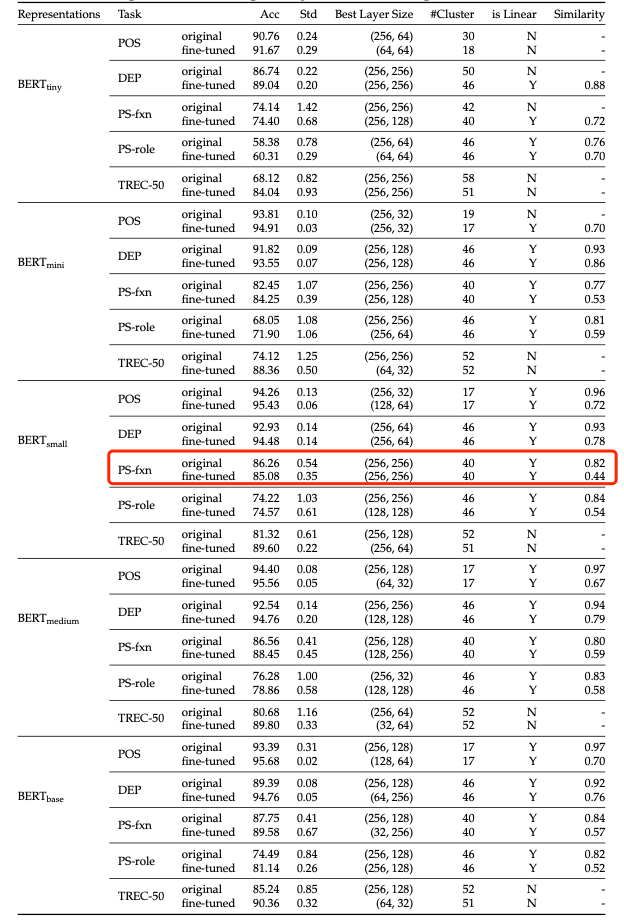
We observe that BERT-small does not show improvments after fine-tuning process on supersense function task, which seems to be odd considering in all other cases, the fine-tuning improves the performance. In the meanwhile, we also obsverve that after fine-tuning, the spaital similarity between training and test set is decreasing for all representations and tasks (showed in the last column), indicating that the training and test sets become divergent as a result of fine-tuning.

Fine-tuning Memorizes Training Set

To understand why BERT-small decreases the performance on the supersense function task, we hypothesize that fine-tuning can memorize the training set. To validate this htpothesis, we design the following experiment:

• We divide the training set into two 80:20 parts, called the subtrain and subtest ses respectively.
• We fine-tuning the representations on the whole training set.
• Then we train a classifier using the subtrain set and test on the subtest and the real test set.

The difference bwtween the subtest and test sets are, subtest is used during fine-tuning but not visible to the classifiers. The following table summarizes the visibility.

The visibility of each subset during fine-tuning and classifiers training

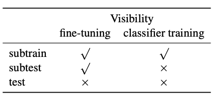
By comparing the learning curves of subtest and test set, we can verify if the fine-tuning process memorizes the subtest. We conduct our experiments on the four tasks using BERT-small. The following figures show the results.

Learning curve comparsions before and after fine-tuning for all four tasks on BERT-small

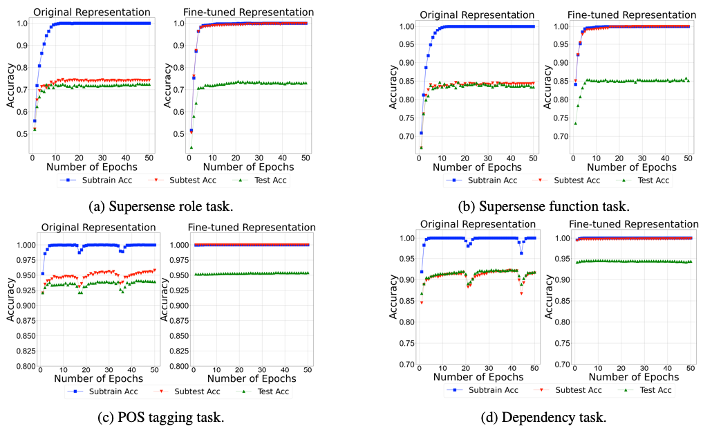
In the above figures, we can observe that before fine-tuning, subtest and test have a similar learning curve; while after fine-tuning, subtrain and subtest have a similar curve although subtest is not visible for classifier training. This observations means that the representation memorizes the subtest during the fine-tuning process such that subtrain and subtest share the exactly the same regularity. Although this observation of memorization cannot explain why BERT does not improve the performance after fine-tuning, it points to a possible direction for investigation: If the memorization beomes severe, will the fine-tuning process overfit the training set and cannot generalize to unseen examples? We leave this question for future research.

Linearity of Representations

After analyzing the performance of fine-tuning, we will take a deeper step to see the geometric change during fine-tuning. In this subsection, we will focus on the linearity of the representations by comparing the number of clusters produced by DirectProbe before and after fine-tuning.

Smaller Representations Require More Complex Classifiers

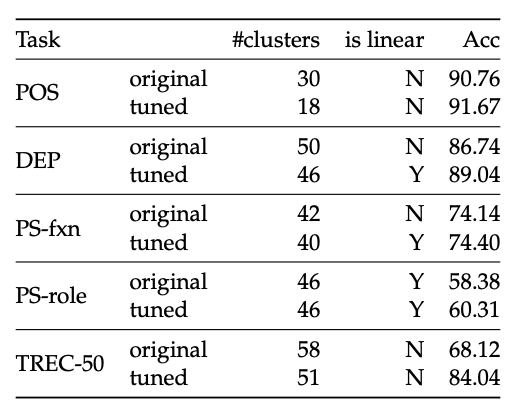
The following table summarizes the results on BERT-tiny. We only show BERt-tiny here because other representations are linearly separable even before fine-tuning. In the following table, we observe that small representations such as BERT-tiny are non-linear for most of the tasks. Although a non-linearity does not necessarily imply poor generalizaiton, it represents a more complex spatial structure and requires a more complex classifier. It would be advisable to use a non-linear classifier if we want to use a small representations (say due to limited resources).

The linearity of the last layer of BERT-tiny for each task

Fine-tuning Makes the Space Simpler

In the above table, we also observe that after fine-tuning, the number of clusters decreases, suggesting that fine-tuning updates the space such that points with different labels are in a simpler spatial configuration.

Spatial Structure of Labels

Next, let’s analyze the spatial structure of the representations during fine-tuning. In this subsection, we focus on tracking the distance between clusters and how these clusters move.

Fine-tuning Pushes Each Label Away From Each Other

We track the minimum distance of each label to all other labels during fine-tuning¹. The following figure shows these distances change in the last layer of BERT-base.

The dynamics of the minimum distance of the three most increased and three least increased labels. The x-axis is the number of fine-tuning updates; the y-axis is chosen label's minimum distance to other labels

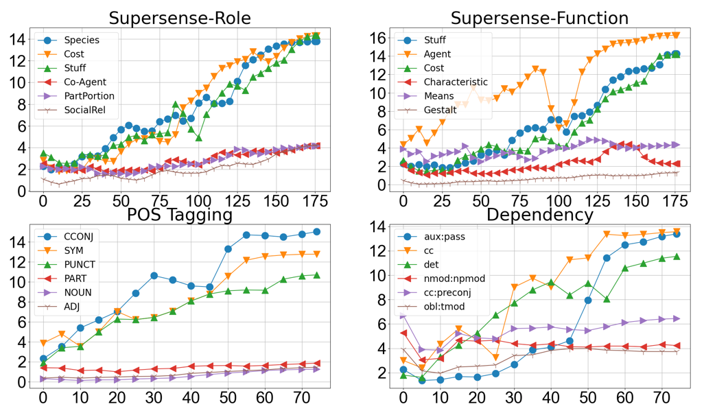
For clearity, we only present the three labels where the mimimum distance increases the most, and three where it increases the least. We also observe that although the trend is increasing, the minimum distance of each label can decrease during the course of fine-tuning, e.g. the label STUFF in supersense role task, suggesting the instability of fine-tuning.

To better understand how these labels move during the fine-tuning, we compute the centroids of each cluster to represent the label position. We select three closest labels from the POS tagging task and track the paths of the centroids of each label cluster in the last layer of BERT-base during the fine-tuning. The following figure shows the PCA projection in 2D of these paths.

The PCA projection of three closest labels in POS tagging task based on the first(left) and last (right) layer of BERT-base.

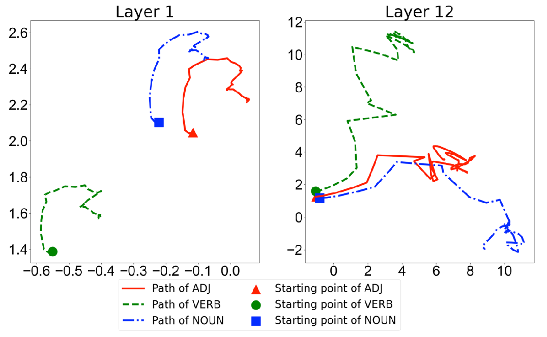
We observe that before fine-tuning, the centroids of all these three labels are close to each other. As the fine-tuning proceeds, the centroids move around in different directions and become far away from each other.

We conclude that fine-tuning pushes each label away from others. This larger gap between labels admits more classifiers consistent with the labels, and allows for better generalization. Note that neither the loss function nor the optimizer explicitly mandates this change. Indeed, since in most cases, the labels are originally linearly separable, the learner need not adjust the representation at all.

Cross-task Fine-tuning

In the last subsection, we hypothesiz that fine-tuning improves the task performance by enlarging the gaps between label clusters. A natural inference of this hypothesis is if we can have a process that shrinks the gaps between labels, we should be able to obersve a decreasing performance. In this subsection, we investigate how fine-tuning for one task affects another.

In this experiment, we fine-tune BERT-base on the PS-role and POS tagging task separately and use the fine-tuned models to generate contextualized representations for the PS-fxn task. We choose PS-role because PS-role and PS-fxn are similar tasks. On the other hand, POS tagging and PS-fxn are contradicting tasks. POS tagging require all the perpositions to be grouped together, while PS-fxn requires differnt prepositions be to far away from each other.

Cross-task fine-tuning results

The above table summarizes our cross-task fine-tuning results. The third and forth columns indicate the number of labels whose minimum distance is increased or decreased after fine-tuning. The second column from the right shows the average distance change over all labels. From this table, we observe that similar tasks (PS-role and PS-fxn) still increases the distance (third row) but in a lesser extent comparing the standarad fine-tuning process (second row). Also, we observe a minor improvements when fine-tuning on a similar task (87.75 –> 88.53). However, when we fine-tuning on a contraticting task, the distances between clusters are all decreasing (last row) and the performance decreases at the same time (87.75 –> 83.24).

In summary, based on the last three subsections, we can conclude that fine-tuning injects or removes task-related information from representation by adjusting the distances between label clusters even if the original representation is linearly separable. When the original representation does not support a linear classifier, fine-tuning tries to group points with the same label into a small number of clusters, ideally one cluster.

Layer Behavior

At last, we will analyze the behaviors of different layers of BERT representation. Previous work has already show that lower layers changed little compared to higher layers. Here, we are going to present more about the layer behaviors.

Higher Layers Change More Than the Lower Layers

First, we quantitatively analyzing the changes to the different layers. We use each cluster’s centroid to represent each label’s position and quantify its movement by computing the Euclidean distance between the centroids before and after fine-tuning for each label, for all layers. Following figure shows movements of POS tagging task using BERT-base.

Euclidean distance between the centroids of labels before and after fine-tuning based on POS tagging task and BERT-base representation. The x-axis is the layer index; the y-axis is the quantified movement, represented by Euclidean distance.

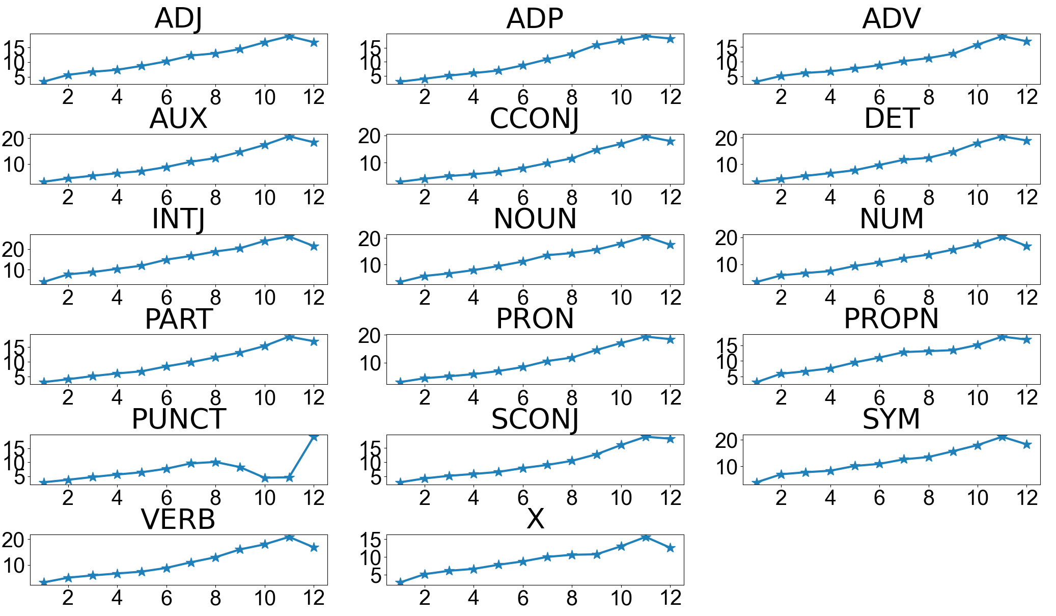
We can observe as the layer increases, the distance becomes larger, suggesting higher layer change more than the lower layers.

Higher Layers Do Not Change Arbitrarily

Although we can confirm that higher layer change more than the lower layers, we find that the hihger layer sitll remain close to the original representations. To study the dynamics of fine-tuning, we compared the intermediate representation of each layer during fine-tuning to its corresponding original pre-trained one. The similarity between two representations is calculated as the Pearson correlation coefficient of their distance vectors as described earlier.

Dynamics of spatial similarity during the fine-tuning process based on BERT-base. The x-axis is the number of gradient updates during the fine-tuning; the y-axis is the Pearson correlation coefficient between current space and its original version.

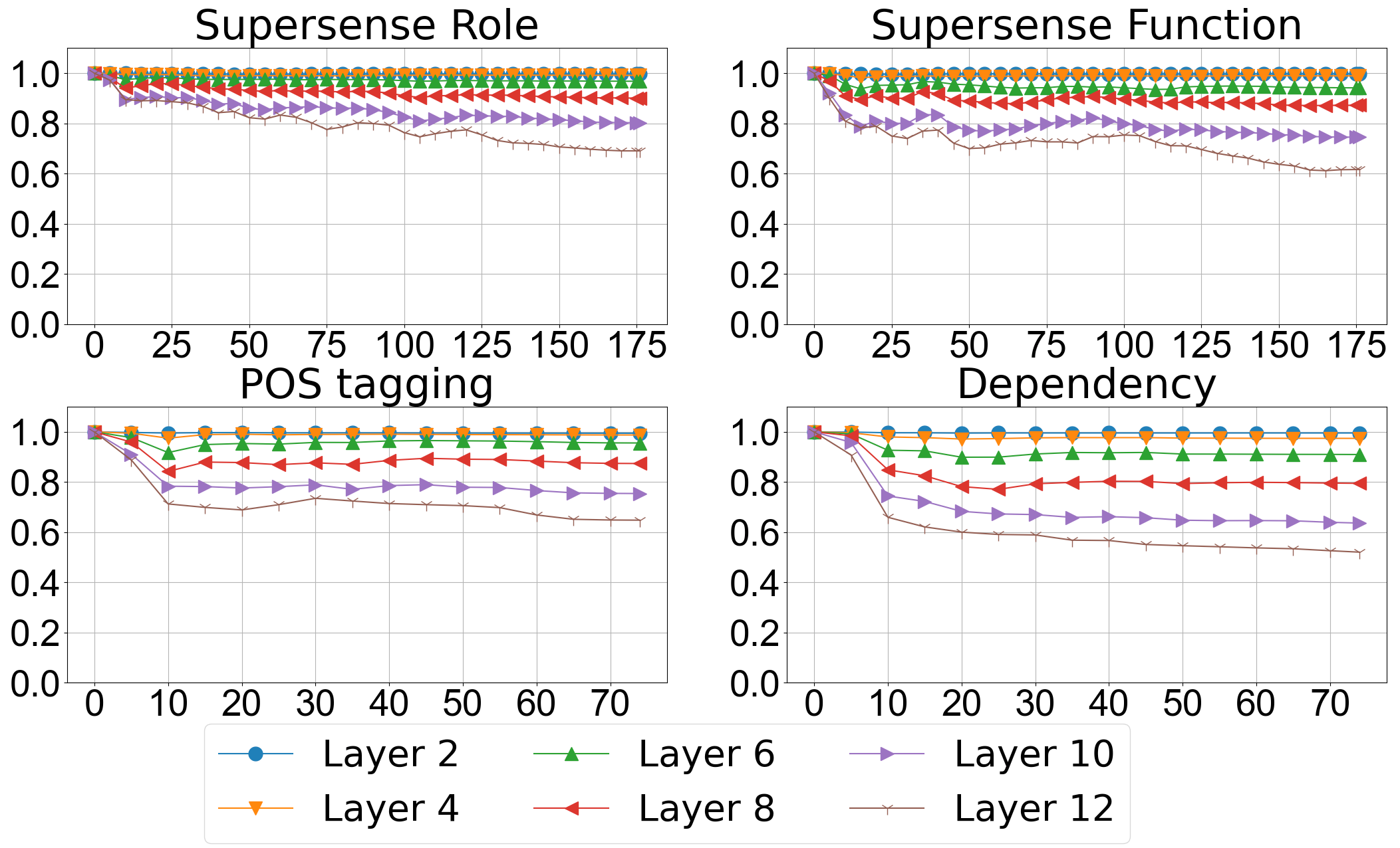
One important observation from the above figure is that even if the higher layers change much more than the lower layers, they do not change arbitrarily. Instead, the high Pearson correlation coefficients of high layers show strong lienar relation (more than $0.5$) between origial representation and the fine-tuned one, suggesting fine-tuning pushes each label away from each other while preserving the relative positions of each label. This means the fine-tuning process encode the task-dependent information while preserving the pre-trained information as much as possible.

The Labels of Lower Layers Move in Small Regions

To verify if the lower layers really do not change, for each label, we compute difference between its centroids before and after fine-tuning. Following figure shows the results.

The PCA projection of the difference vector between centroids of labels before and after fine-tuning based on POS tagging task and BERT-base.

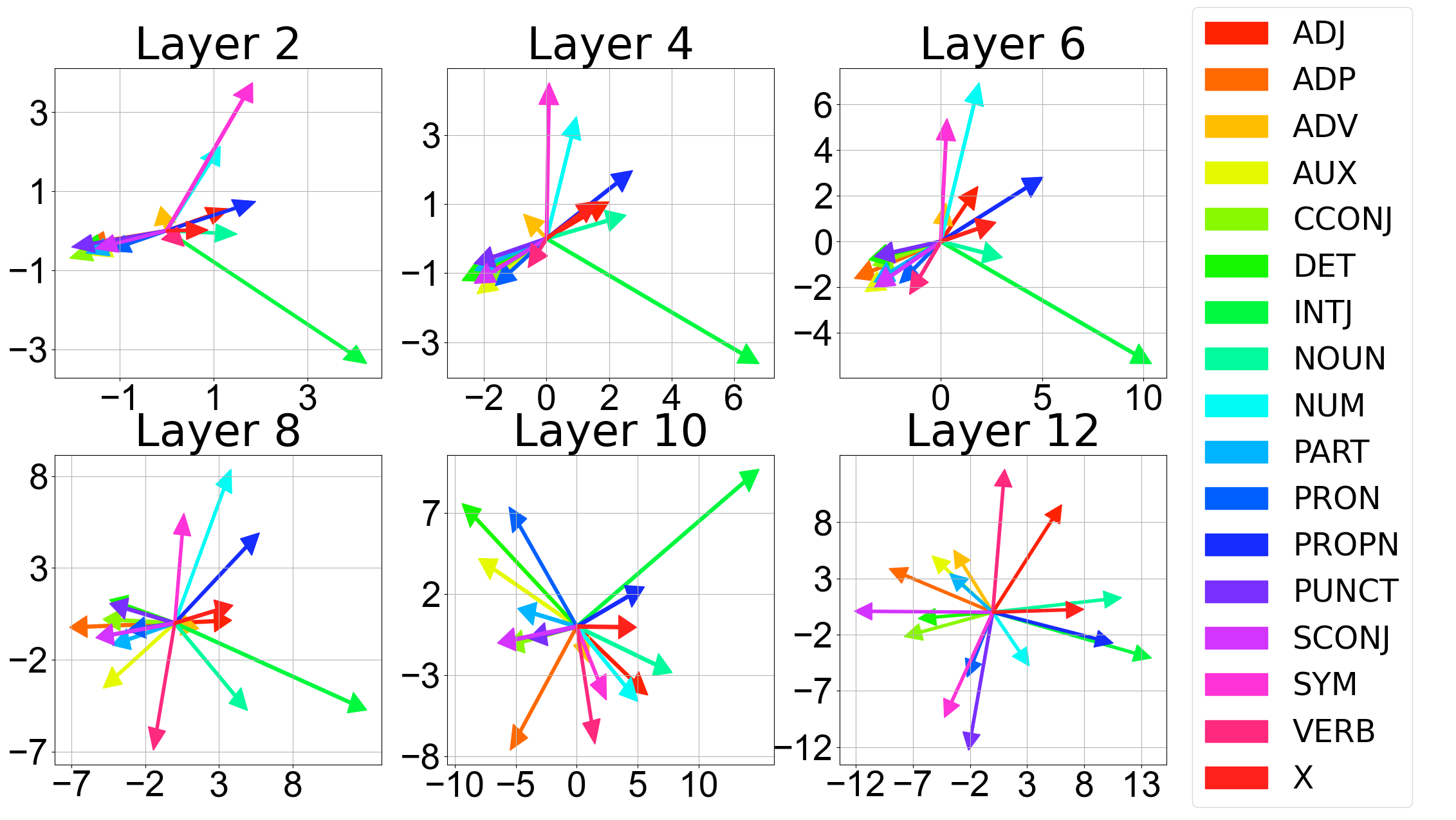
In the above figure, We observe that the movements of labels in lower layers concentrate in a few directions compared to the higher layers, suggesting the labels in lower layers do change, but do not separate the labels as much as the higher layers. Note that, the motion range of lower layers is much smaller than the higher layers. The two projected dimensions range from \(−1\) to \(3\) and from \(−3\) to \(3\) for layer two, while for layer 12 they range from \(−12\) to \(13\) and \(−12\) to \(8\), suggesting that labels in lower layers only move in a small region compared to higher layers.

Conclusion

In this post, we ask and answer the following three questions:

• Does fine-tuning always improve performance?
  • Indeed, fine-tuning almost always improves task performacne. However, rare cases exist where fine-tuning decreases the performance.
  • We also observe a divergence between training and test set after fine-tuning.
• How does fine-tuning alter the representation to adjust for downstream tasks?
  • Fine-tuning alters the representation by grouping points with the same label into small number of clusters;
  • And pushing each label cluster away from each other.
• How does fine-tuning change the underlying geometric structure of different layers?
  • Higher layers do not change arbitrarily, instead, they remain simialr to the untuned vrsion.

1. In most cases, the number of clusters equal to the number of labels. So, we use the clusters and labels interchangeablly. ↩